Examples

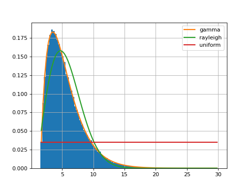
Let us start with an example. We generate a vector of values from a gamma distribution.

from scipy import stats
data = stats.gamma.rvs(2, loc=1.5, scale=2, size=100000)

from fitter import Fitter
f = Fitter(data, distributions=['gamma', 'rayleigh', 'uniform'])
f.fit()
f.summary()

(Source code, png, hires.png, pdf)

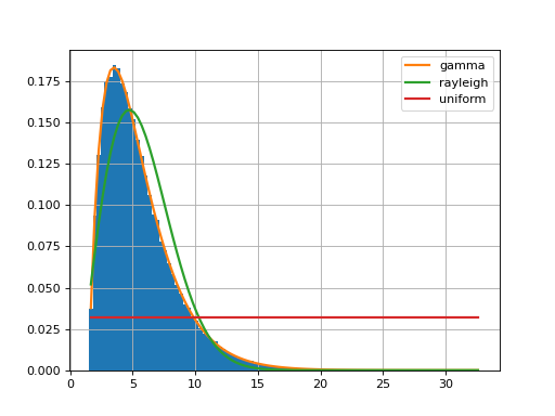
Here, we restrict the analysis to only 3 distributions by providing the list of distributions to consider. If you do not provide that parameter, 80 distributions will be considered (the analysis will be longer) and computation make take a while to finish.

The fitter.fitter.Fitter.summary() method shows the first best distributions (in terms of fitting).

Once the fitting is performed, one may want to get the parameters corresponding to the best distribution. The parameters are stored in fitted_param. For instance in the example above, the summary told us that the Gamma distribution has the best fit. You would retrieve the parameters of the Gamma distribution as follows:

>>> f.fitted_param['gamma']
(1.9870244799532322, 1.5026555566189543, 2.0174462493492964)

Here, you will need to look at scipy documentation to figure out what are those parameters (mean, sigma, shape, …). For convenience, we do provide the corresponding PDF:

f.fitted_pdf['gamma']

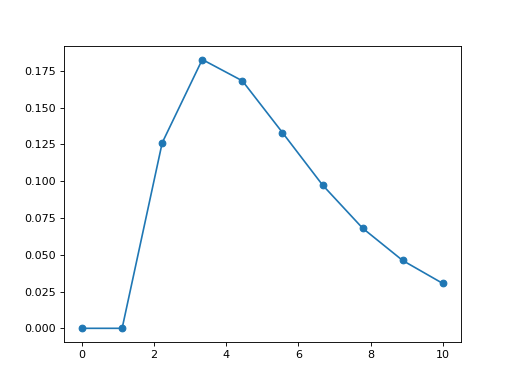
but you may want to plot the gamma distribution yourself. In that case, you will need to use Scipy package itself. Here is an example

from pylab import linspace, plot
import scipy.stats

dist = scipy.stats.gamma
param = (1.9870, 1.5026, 2.0174)
X = linspace(0,10, 10)
pdf_fitted = dist.pdf(X, *param)
plot(X, pdf_fitted, 'o-')

(Source code, png, hires.png, pdf)

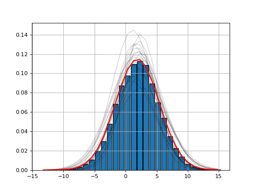
HistFit class: fit the density function itself

Sometimes, you only have the distribution itself. For instance:

import scipy.stats
data = [scipy.stats.norm.rvs(2,3.4) for x in  range(10000)]
Y, X, _ = hist(data, bins=30)

here we have only access to Y (and X).

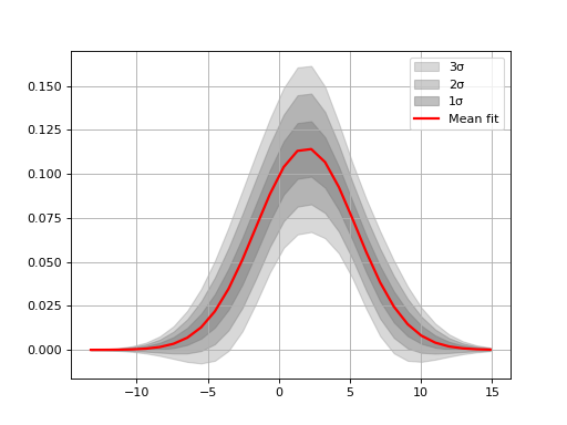
The histfit module provides the HistFit class to generate plots of your data with a fitting curve based on several attempt at fitting your X/Y data with some errors on the data set. For instance here below, we introduce 3% of errors and fit the data 20 times to see if the fit makes sense.

from fitter import HistFit
from pylab import hist
import scipy.stats
data = [scipy.stats.norm.rvs(2,3.4) for x in  range(10000)]
Y, X, _ = hist(data, bins=30)
hf = HistFit(X=X, Y=Y)
hf.fit(error_rate=0.03, Nfit=20)
print(hf.mu, hf.sigma, hf.amplitude)

(Source code)

(png, hires.png, pdf)

(png, hires.png, pdf)