fitter module reference
main module of the fitter package
- class fitter.fitter.Fitter(data, xmin=None, xmax=None, bins=100, distributions=None, timeout=30, density=True)[source]
Fit a data sample to known distributions
A naive approach often performed to figure out the undelying distribution that could have generated a data set, is to compare the histogram of the data with a PDF (probability distribution function) of a known distribution (e.g., normal).
Yet, the parameters of the distribution are not known and there are lots of distributions. Therefore, an automatic way to fit many distributions to the data would be useful, which is what is implemented here.
Given a data sample, we use the fit method of SciPy to extract the parameters of that distribution that best fit the data. We repeat this for all available distributions. Finally, we provide a summary so that one can see the quality of the fit for those distributions
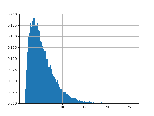
Here is an example where we generate a sample from a gamma distribution.
>>> # First, we create a data sample following a Gamma distribution
>>> from scipy import stats
>>> data = stats.gamma.rvs(2, loc=1.5, scale=2, size=20000)

>>> # We then create the Fitter object
>>> import fitter
>>> f = fitter.Fitter(data)

>>> # just a trick to use only 10 distributions instead of 80 to speed up the fitting
>>> f.distributions = f.distributions[0:10] + ['gamma']

>>> # fit and plot
>>> f.fit()
>>> f.summary()

              sumsquare_error     aic            bic     kl_div  ks_statistic  ks_pvalue
loggamma            0.001176  995.866732 -159536.164644     inf      0.008459   0.469031
gennorm             0.001181  993.145832 -159489.437372     inf      0.006833   0.736164
norm                0.001189  992.975187 -159427.247523     inf      0.007138   0.685416
truncnorm           0.001189  996.975182 -159408.826771     inf      0.007138   0.685416
crystalball         0.001189  996.975078 -159408.821960     inf      0.007138   0.685434
Once the data has been fitted, the
summary()method returns a sorted dataframe where the index represents the distribution names.The AIC is computed using
 ,
and the BIC is computed as
,
and the BIC is computed as 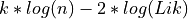 .
.where Lik is the maximized value of the likelihood function of the model, n the number of data point and k the number of parameter.
Looping over the 80 distributions in SciPy could takes some times so you can overwrite the
distributionswith a subset if you want. In order to reload all distributions, callload_all_distributions().Some distributions do not converge when fitting. There is a timeout of 30 seconds after which the fitting procedure is cancelled. You can change this
timeoutattribute if needed.If the histogram of the data has outlier of very long tails, you may want to increase the
binsbinning or to ignore data below or above a certain range. This can be achieved by setting thexminandxmaxattributes. If you set xmin, you can come back to the original data by setting xmin to None (same for xmax) or just recreate an instance.- distributions
list of distributions to test
- fit(progress=False, n_jobs=-1, max_workers=-1, prefer='processes')[source]
Loop over distributions and find best parameter to fit the data for each
When a distribution is fitted onto the data, we populate a set of dataframes:
df_errors:sum of the square errors between the data and the fitted distribution i.e.,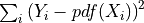
fitted_param: the parameters that best fit the datafitted_pdf: the PDF generated with the parameters that best fit the data
Indices of the dataframes contains the name of the distribution.
- get_best(method='sumsquare_error')[source]
Return best fitted distribution and its parameters
a dictionary with one key (the distribution name) and its parameters
- plot_pdf(names=None, Nbest=5, lw=2, method='sumsquare_error')[source]
Plots Probability density functions of the distributions
- Parameters:
names (str,list) – names can be a single distribution name, or a list of distribution names, or kept as None, in which case, the first Nbest distribution will be taken (default to best 5)
- summary(Nbest=5, lw=2, plot=True, method='sumsquare_error', clf=True)[source]
Plots the distribution of the data and N best distributions
- property xmax
consider only data below xmax. reset if None
- property xmin
consider only data above xmin. reset if None

histfit module reference
- class fitter.histfit.HistFit(data=None, X=None, Y=None, bins=None)[source]
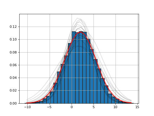
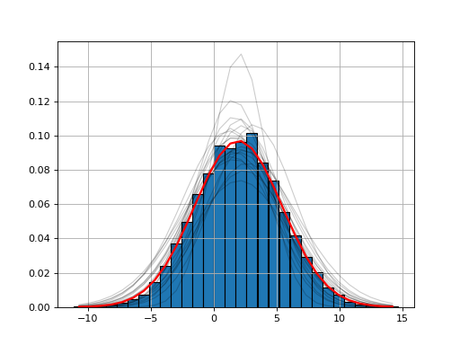
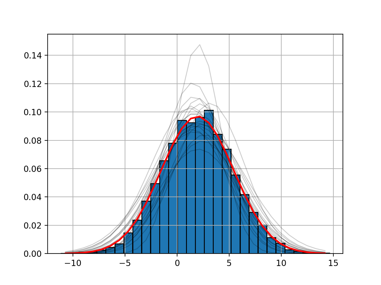
Plot the histogram of the data (barplot) and the fitted histogram (gaussian case only)
The input data can be a series. In this case, we compute the histogram. Then, we fit a curve on top on the histogram that best fit the histogram.
If you already have the histogram, you can provide the density function.. In such case, we assume the data to be evenly spaced from 1 to N.
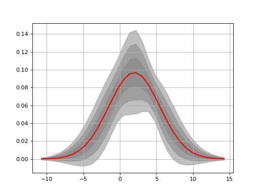
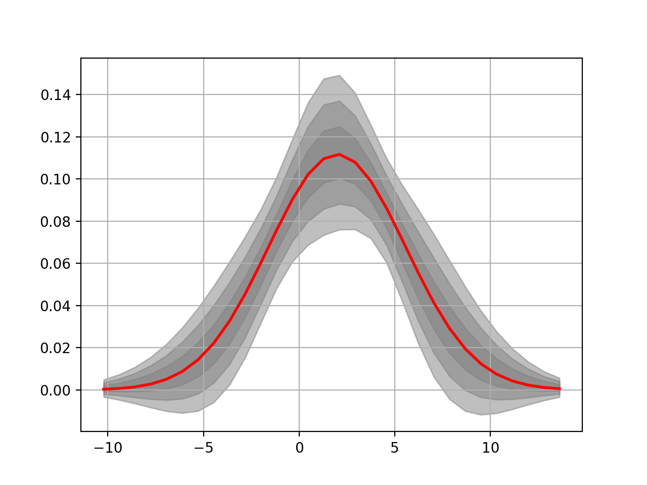
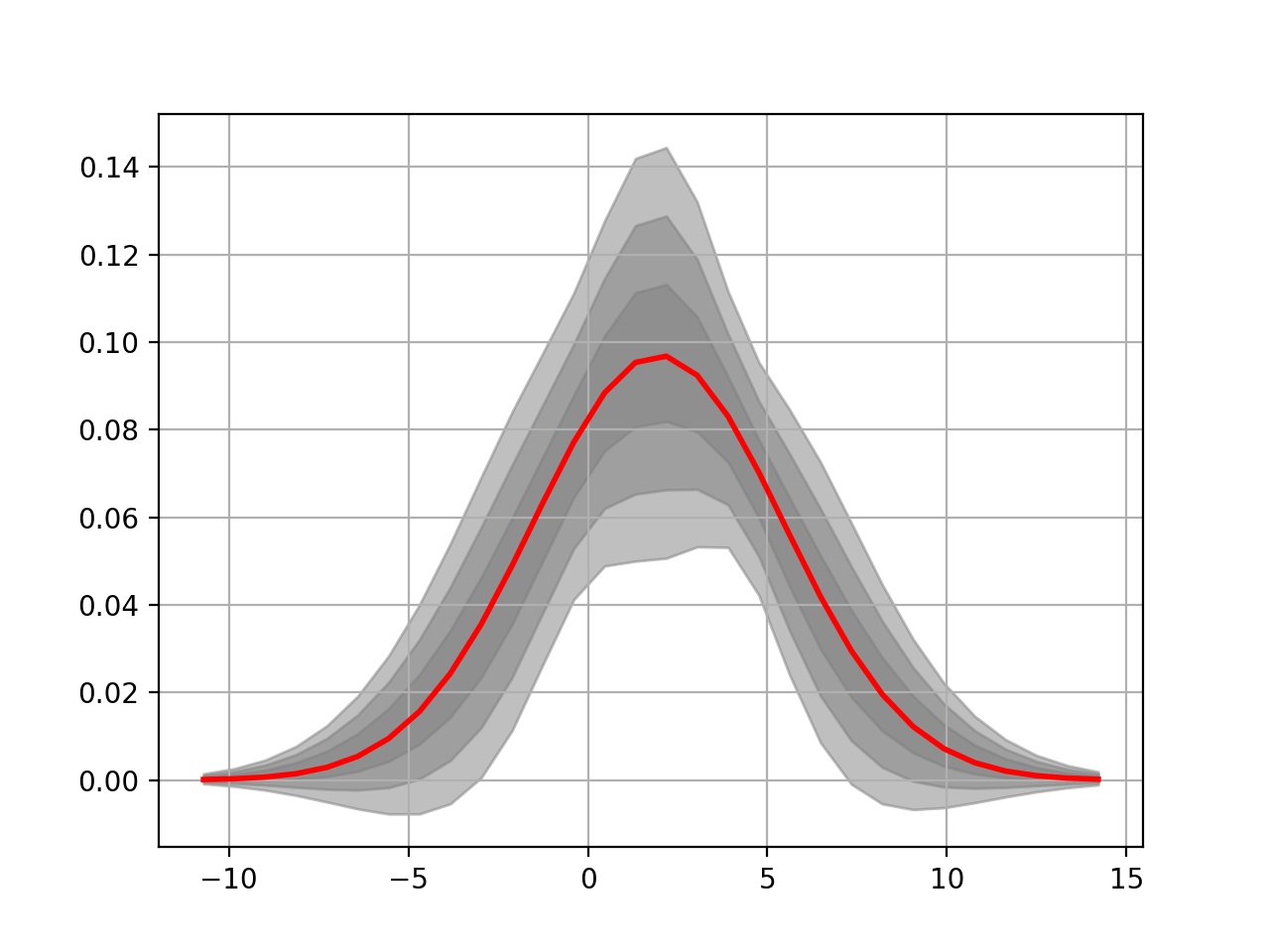
If you have some data, histogram is computed, then we add some noise during the fitting process and repeat the process Nfit=20 times. This gives us a better estimate of the underlying mu and sigma parameters of the distribution.

You may already have your probability density function with the X and Y series. If so, just provide them; Note that the output of the hist function returns an X with N+1 values while Y has only N values. We take care of that.
Warning
This is a draft class. It currently handles only gaussian distribution. The API is probably going to change in the close future.
